A few months ago, I played Hunt: Showdown, a competitive multiplayer shooter produced by Crytek. Hunt is an unusual game in which teams of one, two, and three players all compete for the same objectives. How can such a design ever be well-balanced for a competitive game?
Hunt: Showdown balances asymmetrical teams by ensuring that smaller teams play against worse players to compensate for the disadvantage of having fewer teammates.
While explaining Hunt: Showdown to a friend, we weren’t sure whether that second point is fair in practice; is it reasonable for the game’s rating system to pit a single seasoned gamer against a team of newbies? I set out to answer this question.
Rating System
Hunt: Showdown uses an Elo rating system (also known as Match Making Rating or “MMR"). Whenever a player kills another player, both players' MMRs are updated. Instead of exposing each player’s 4-digit MMR, each player is grouped into a broader “star rating” between 1 (the lowest rating) and 6 (the highest rating).
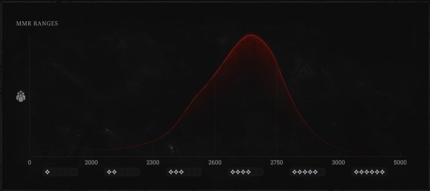
These individual MMR scores are then used to calculate a “Match MMR”. Match MMR is explained by Hunt: Showdown as follows:
Match MMR is a score used for team matchmaking. Match MMR takes each team member’s individual MMR and uses it to calculate a team MMR score. This value - your team’s Match MMR - is then used to find a fitting match. Additional modifiers can be applied on top to help place smaller or random teams in fairer matches.
In short, solo players will have a lower Match MMR, allowing them to be matched against other solo players of similar skill and teams of players who are individually weaker.
Modelling the Encounter
To mathematically model an encounter between two differently-sized, differently-skilled teams, we’ll use a Markov chain. We’ll then use our model to calculate the probability of each team winning.
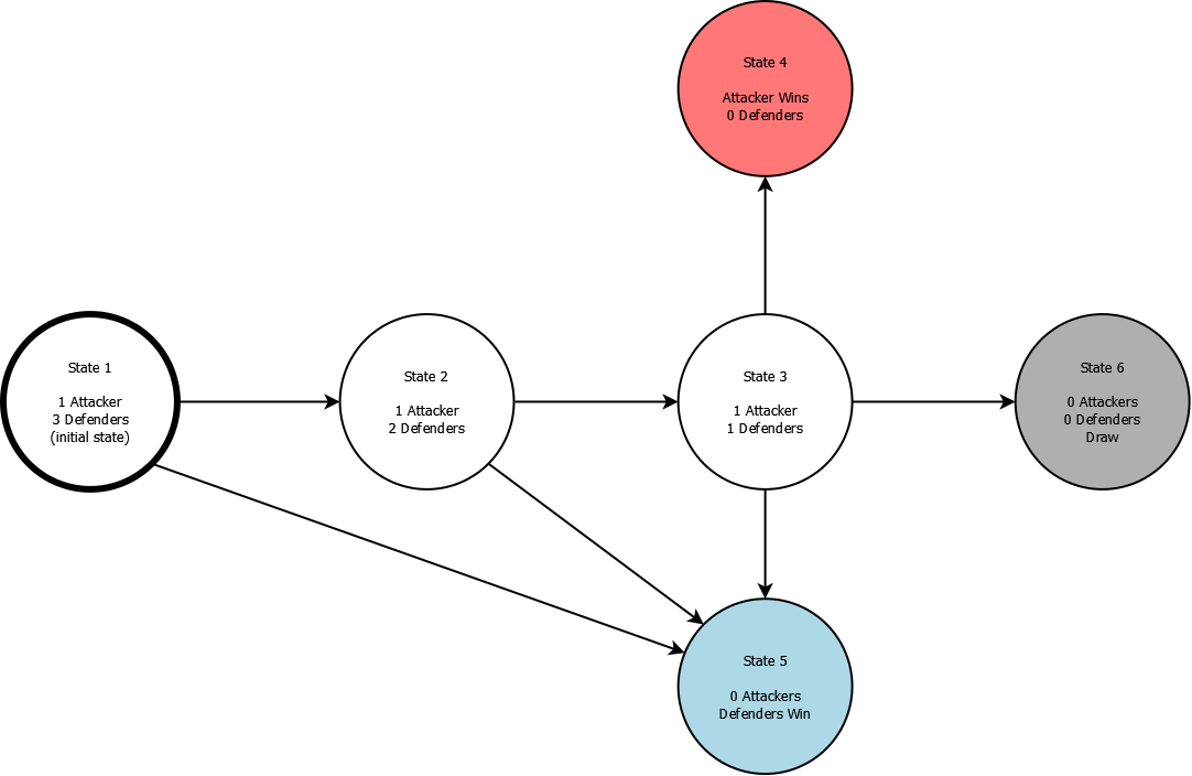
To start building the Markov chain, we need a list of states. As an example, we’ll list all the relevant states in a fight between 1 attacker and 3 defenders. These are:
- 1 attacker alive, 3 defenders alive
- 1 attacker alive, 2 defenders alive
- 1 attacker alive, 1 defender alive
- 0 attackers alive (defenders win)
- 0 defenders alive (attackers win)
- Nobody left alive (draw)
We also need a list of transitions which model how the encounter can move between these states. To simplify the Markov chain, we’ll make a few assumptions:
- Dead players cannot be revived by teammates
- A maximum of one player from each team can die at a time
With those assumptions in mind, here is a diagram showing the 6 states (the circles) and the transitions between them (the arrows):
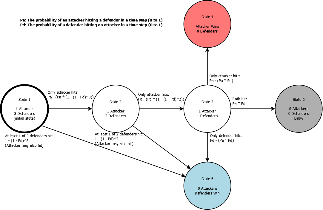
Our model starts in State 1, and advances in discrete, fixed increments (also known as “time steps”). We need to do some math to identify the probability of each transition occurring in a given time step. In particular, we would like to be able to express these probabilities in terms of each player’s skill.
To quantify the skill of the attackers and defenders, we will define the following terms:
- Pa: The probability of an attacker killing a defender in a time step (0 to 1)
- Pd: The probability of a defender killing an attacker in a time step (0 to 1)
We’d like to come up with equations which represent the probability of each transition occurring in terms of Pa and Pd. For instance, here is the probability of each transition starting from State 3 (1 attacker and 1 defender).
- State 4 (attackers win): Pa - (Pa * Pd) (only the attacker hits)
- State 5 (defenders win): Pd - (Pa * Pd) (only the defender hits)
- State 6 (draw): Pa * Pd (both players hit each other)
The probabilities for every transition in the diagram can be calculated using similar logic. Here is the same diagram as above, but with all probabilities labelled in terms of Pa and Pd:
With these equations, our model of the encounter is complete, and we can start programming.
Running the Model
Running calculations on our Markov chain will require a good deal of matrix arithmetic. Python supports these operations with the NumPy and pandas packages, so Python is a natural choice for this project.
Our first step is to take the previously-derived equations and turn them into a probability matrix. Each row of this matrix contains the probabilities (from 0 to 1) of transitioning from one state to every other state. Because our Markov chain has 6 states, our probability matrix will have 6 rows and 6 columns. For instance, the 6th entry in the 3rd row of the matrix represents the probability of transitioning from State 3 to State 6.
Since our equations were defined in terms of Pa and Pd, so we will write a function that takes Pa and Pd to return the probability matrix (implemented as a NumPy array):
import numpy as np


def get_probability_matrix(pa, pd):
    """
    Given pa and pd, returns the probability matrix.
    :param pa: The probability of an attacker killing a defender in a time step (0 to 1)
    :param pd: The probability of a defender killing an attacker in a time step (0 to 1)
    :return: The probability matrix (NumPy array)
    """
    s_1_to_5 = 1 - (1 - pd) ** 3
    s_2_to_5 = 1 - (1 - pd) ** 2
    return np.array([
        [(1 - pa) * (1 - s_1_to_5), pa - (pa * s_1_to_5), 0, 0, s_1_to_5, 0],  # state 1
        [0, (1 - pa) * (1 - s_2_to_5), pa - (pa * s_2_to_5), 0, s_2_to_5, 0],  # state 2
        [0, 0, (1 - pa) * (1 - pd), pa - (pa * pd), pd - (pa * pd), pa * pd],  # state 3
        [0, 0, 0, 1, 0, 0],  # state 4
        [0, 0, 0, 0, 1, 0],  # state 5
        [0, 0, 0, 0, 0, 1],  # state 6
    ])
This matrix contains the same equations we derived above expressed in Python code. Note that there are no transitions away from States 4, 5, or 6; these are the end states of the encounter. We should also initialize a 1 by 6 array that holds the initial state:
INITIAL_STATE = np.array([[1, 0, 0, 0, 0, 0]]) # we start the encounter at State 1 of 6
Now that we have our probability matrix and an initial state, we’ll need a function that runs the model. Advancing the state of the model by one time step can be accomplished by taking the dot product of the current state with the probability matrix.
def run_simulation(initial_state, probability_matrix, num_steps):
    """
    Simulates a Markov chain for a certain number of steps.
    :param initial_state: The initial state of the simulation (NumPy array)
    :param probability_matrix: The probability matrix (NumPy array)
    :param num_steps: The number of steps to run the simulation
    :return: The history of all states in the simulation (NumPy array)
    """
    history = initial_state  # initialize state history with the initial state
    current_state = initial_state  # initialize current state with the initial state

    for _ in range(num_steps):
        current_state = np.dot(current_state, probability_matrix)  # advance state
        history = np.append(history, current_state, axis=0)  # add new state to history

    return history
We’ll use pandas to automatically generate a nicely-formatted area plot from the simulation’s history data:
import pandas


def show_plot(history, title):
    """
    Plots the simulation history of the Markov chain simulation.
    :param history: The simulation history (NumPy array)
    :param title: The title for the plot
    """
    df = pandas.DataFrame({
        'State 1 (1 vs 3)': history.T[0],
        'State 2 (1 vs 2)': history.T[1],
        'State 3 (1 vs 1)': history.T[2],
        'State 4 (attacker wins)': history.T[3],
        'State 5 (defenders win)': history.T[4],
        'State 6 (draw)': history.T[5],
    })
    df.plot.area(
        xlabel='Elapsed time steps',
        ylabel='Probability',
        title=title,
    )
    plt.show()
Finally, we’ll add a few lines of code that call all these functions: getting the probability matrix, using the probability matrix to run the simulation, and plotting the simulation’s history:
NUM_ITERATIONS = 150  # number of time steps to run the simulation

PROB_ATTACKER_HITS = 0.05  # Pa
PROB_DEFENDER_HITS = 0.05  # Pd

prob_matrix = get_probability_matrix(PROB_ATTACKER_HITS, PROB_DEFENDER_HITS)
state_history = run_simulation(INITIAL_STATE, prob_matrix, NUM_ITERATIONS)

plot_title = '1v3 probability with Pa = {0} and Pd = {1}'.format(PROB_ATTACKER_HITS, PROB_DEFENDER_HITS)
show_plot(state_history, plot_title)
Now that we have all this code, we’re ready to run our model and obtain some meaningful results.
Results and Analysis
Let’s examine a simple case where every player on the differently-sized teams is equally skilled (i.e. Pa = Pd). We could use any value between 0 and 1, but for now we’ll set both Pa and Pd to 0.05 so that each player has a 5% chance of hitting an opposing player every time step. To give the encounter sufficient time to resolve, we’ll run the simulation for 150 time steps.
In this case, you would expect the defenders to emerge victorious most of the time since they have a larger team. This outcome is exactly what we can see in the simulation when setting Pa and Pd to 0.05:
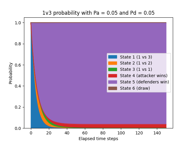
In this instance, the defenders emerge victorious 96.2% of the time while the lone attacker wins 3.6% of the time. It’s intuitively clear that it’s better to have more teammates on the field, but this example illustrates how the advantage is overwhelming.
To compensate for this advantage, let’s make each individual player on the defending team less skilled. We’ll set Pd to 0.01, so each defender only has a 1% chance of hitting the attacker every time step, while Pa will stay at 0.05.
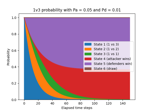
This change was quite drastic, but it seemed to give the lone attacker a fighting chance. The attacker’s odds of winning are now 36.6% while the defenders' are 62.9%.
Even though the attacker is 5 times “better” than each of the 3 defenders individually, the defenders are still heavily favoured to win. This discrepancy occurs because the 3 defenders have many more opportunities to hit the lone attacker by virtue of having more players on their team.
This effect can be clearly seen by setting Pa to 1, representing an encounter where the attacker never misses:
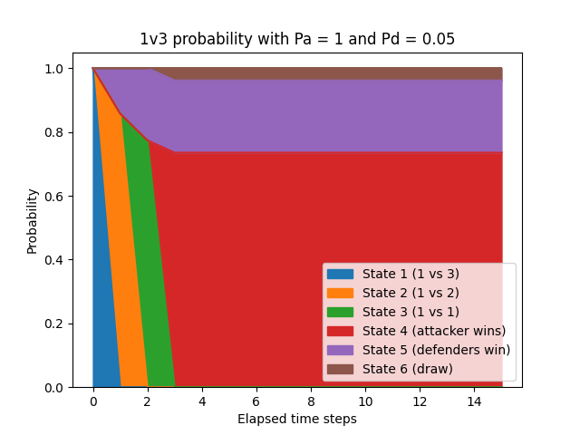
The assumption that a player would never miss is not realistic. That said, even when the attacker is guaranteed to hit, the defenders (who only have a 5% chance to hit) still get plenty of opportunities to hit the attacker - and they only need to get lucky once. In the graph above, the attacker’s odds of winning are 73.5% and the defenders' are 22.6%. (The odds of a draw are relatively high, with a 3.9% chance that both of the last two players hit each other at the same time.)
We can also use the model to simulate an asymmetrical 1v2 encounter by setting the initial state of the Markov chain to State 2:
INITIAL_STATE = np.array([[0, 1, 0, 0, 0, 0]])
With that change, let’s run this simulation with the same parameters as before:
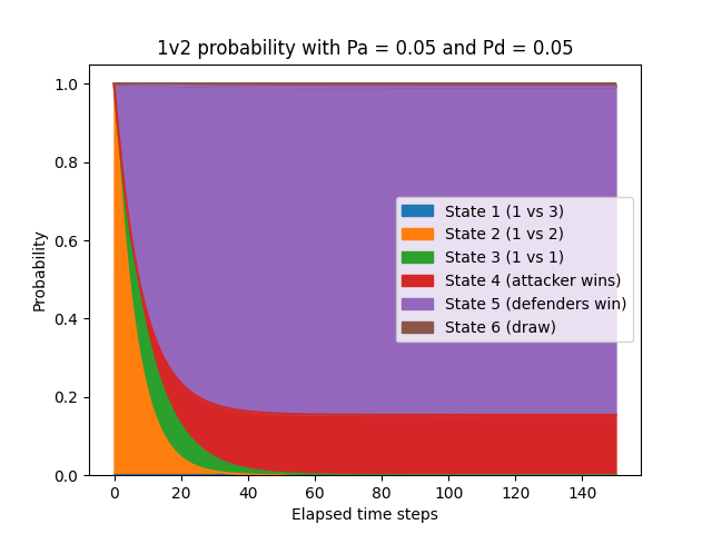
- Probability of attacker winning: 15.4% (up from 3.6%)
- Probability of defenders winning: 83.8% (down from 96.2%)
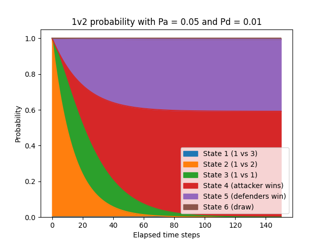
- Probability of attacker winning: 59.1% (up from 36.6%)
- Probability of defenders winning: 40.2% (down from 62.9%)
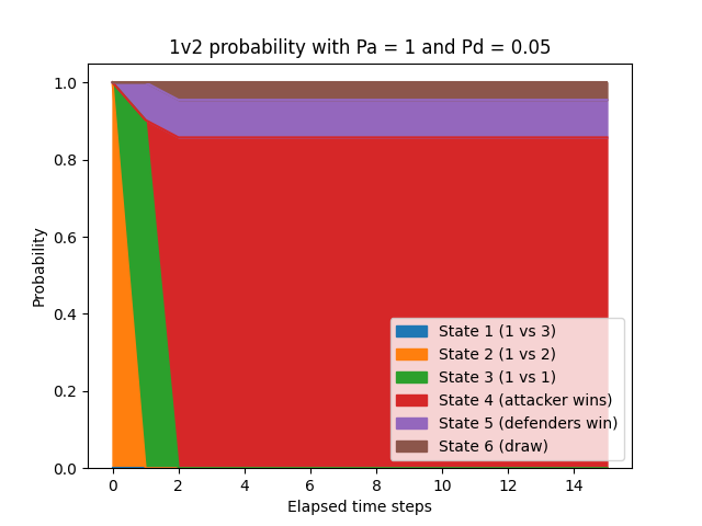
- Probability of attacker winning: 85.7% (up from 73.5%)
- Probability of defenders winning: 9.8% (down from 22.6%)
- Probability of drawing: 4.5% (up from 3.9%)
As one would expect, the lone attacker’s odds of winning go up when the defenders have fewer team members.
Conclusion
Asymmetric team sizes can generally be balanced by matching higher-skilled players against larger teams. However, having a larger team is a huge advantage: even when a lone attacker is five times more skilled than any of three defenders, the defenders are still favoured to win through sheer numbers.
Anecdotally, while playing Hunt: Showdown, the maximum I have seen a player’s Match MRR be adjusted by is 1 out of 6 stars. The skill difference this one-star change represents is substantial, but so are the advantages afforded by having a larger team: we’ve seen how a group of less-skilled players can easily overpower a single skilled player.
Without access to the game’s backend matchmaking data, we cannot definitively identify whether the adjustments made by Hunt: Showdown are sufficient to overcome the advantage of having more teammates. However, we’ve seen that the general principle is sound, so while the implementation of the system in Hunt: Showdown may not go far enough, the system still nudges fights in the right direction.
Acknowledgements
- Violet Adrasteia Dawn (for initially sparking this discussion)
- Jonah Cowan (for proofreading and editing)
- Laura McLean (for proofreading and editing)